
Eddyfi Technologies has implemented a new data acquisition technique for TFM called Plane Wave Imaging (PWI) in Capture™ 3.1 software. This technology was developed to improve productivity and sensitivity which are sometimes seen as some drawbacks of the Total Focusing Method (TFM). PWI combines the commonality of a sectorial scan used for PAUT with the optimum spatial resolution of TFM. We shared how to define a proper scan plan to ensure full coverage of a weld under inspection in an earlier blog and YouTube video.
PWI not only improves scanning speed and the energy sent into a test piece but also records the elementary signals used to create the TFM image at a significant rate within an acceptable data file size. This blog is dedicated to the analysis of PWI inspection files.
TFM was first introduced as a post-processing technique. Inspectors were acquiring elementary Full Matrix Capture (FMC) data using a phased array system, transferring the data to a computer and then calculating the TFM images. While powerful, the technique was only used in laboratories due to the time-consuming process. The apparition of systems capable of providing TFM in real-time, like the M2M Gekko®, allowed the technique to be used in the field for the first time.
While all Phased Array Ultrasonic Testing (PAUT) systems developed by Eddyfi Technologies (Mantis™, Gekko, and Panther™) can save elementary FMC data, it usually isn’t kept as the amount of data generated is quite large. For example, in the blog about the scan plan, we performed an acquisition on a 300-millimeter (11.8-inch) long, 25 mm (1 in) V-weld acquiring data points every millimeter (0.04 in) using a 5-MHz 64-element probe sampled at 33.3 MHz. Acquiring the elementary FMC data (64 x 64 = 4096 signals) on top of the TFM would increase the file size from 185 MB to 3.9 GB. If we extrapolate to a 500 mm (20 in) pipe, it would result in a file of 20 GB which is not realistic to manage.
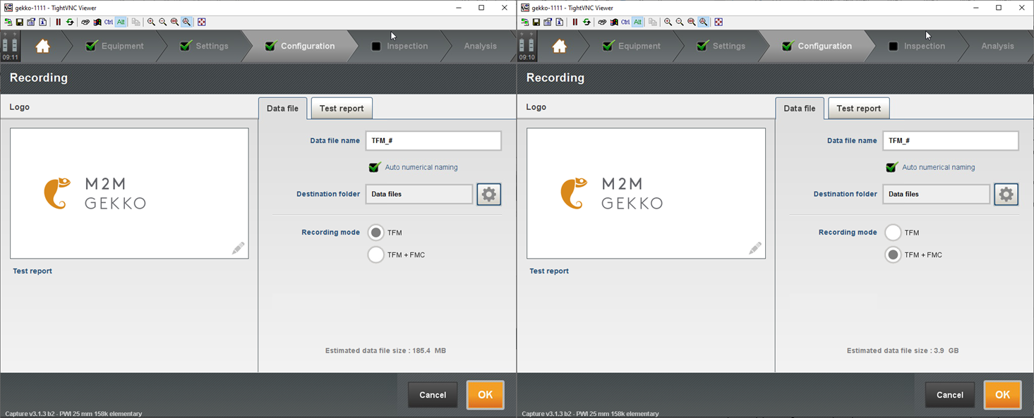
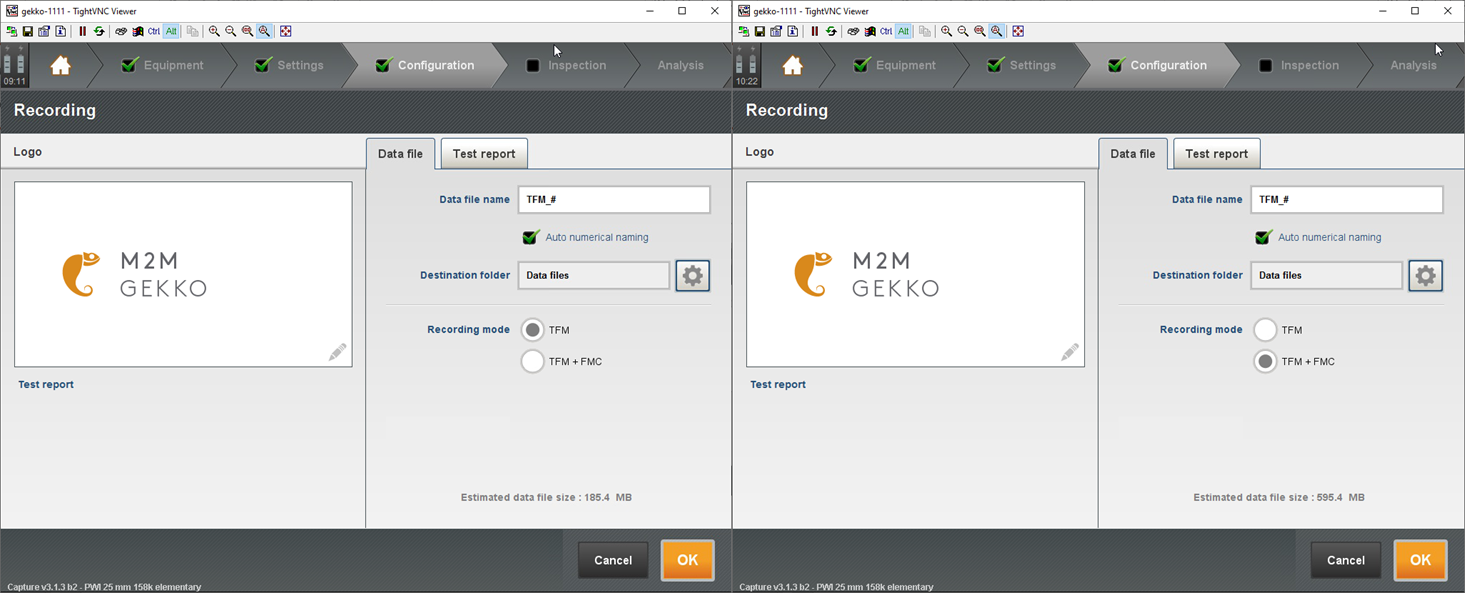
PWI, on the other hand, generates less data. The PWI process was described in this blog. Essentially, we use a phased array probe with N elements and perform a sectorial scan along a few angles M for the excitation. At the end of the PWI data acquisition process, the resulting matrix contains M × N elementary A-Scans compared to N x N for elementary FMC. Going back to the weld example, the file size would go from 185 MB to 595 MB. For a 500 mm (20 in) pipe, it would generate a 3 GB file which is still big but more manageable.
Acquiring elementary data around indications may be of interest when operators find anomalies during their initial scan. This would offer small files for experts to analyze defects afterwards.
Post-processing Examples
There are several reasons for which one would like to save the elementary data, including but not limited to:
- Changing the position and size of the TFM image after the acquisition;
- Adjusting the number of pixels;
- Calculating different modes that were not acquired during scanning;
- Changing the thickness or the geometry completely;
- Changing the material properties of the component.
Eddyfi Technologies can provide customers with a library so they can develop their software to process FMC data; contact us for more information. Watch this video for an example of FMC data read in Excel and TFM calculated using Python post-processing.
Capture software files are also compatible with CIVA and CIVA Analysis. We use CIVA Analysis here to illustrate the various examples described before.
Change the Position of the TFM Image and the Number of Pixels After the Acquisition
In a previous blog, we optimize the PWI/TFM parameters (ROI size and position, number of pixels, etc.) to have the best scanning speed while maintaining code compliance. We rescan the plate and acquire the PWI elementary data. We post-process it —changing the size and position of the ROI to start from the front surface— and increase the number of pixels to 316 kpixels. Post-processing the 300 mechanical positions of the scan takes about 1’30 with a laptop with a i7-8750H processor. With a newer CPU, we could process a 500 mm (20 in) weld within a few minutes.
Calculate Various Modes
One of the advantages of TFM is the ability to detect defects through a multiplicity of paths or modes. Using the specimen boundaries, it’s possible to view indications from different directions while accounting for mode conversion. In our weld example, we acquire the T-T and TT-TT simultaneously, which allows us to see all the defects from both sides. The more modes we add during the acquisition, the slower the scanning speed as the system processes more data. It’s also not possible to predict all the defect orientations beforehand, so being able to post-process any mode is beneficial. In the following video, we post-process the previous data to calculate the TT, TTT, TTTT, TTTTT modes and look at the three defects with the various modes.
Change the Velocity
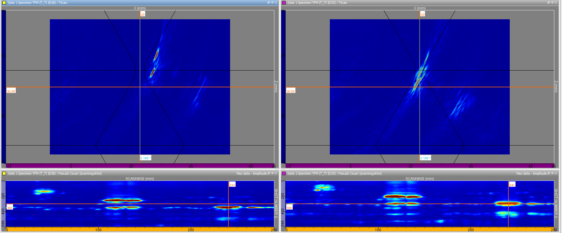
When scanning components, it’s possible to have an inexact value for material velocity. Using the wrong velocity leads to a shift in position and change in amplitude. The following images show the root crack for a velocity of 3230 m/s on the left and 3100 m/s on the right. We can see the root crack not positioned correctly and lose the two original echoes.
This feature is already available with Acquire™ software used with the Panther desktop system. With the release of Plane Wave Imaging in Capture 3.1, saving elementary data is now a faster process that also provides reasonable data file sizes for efficient operations in the field. This feature is especially useful for people who want to modify the parameters (geometry, velocity, ROI, etc.) of their inspection after the fact.
Learn more about this feature and the many more offered by our advanced PWI/TFM instruments by contacting our experts today, and subscribe to our blog to receive articles like this direct to your inbox!