
Originally designed for detecting Corrosion Under Insulation (CUI) in petrochemical plant pipework, Guided Wave Testing (GWT) with the Teletest Focus+™ has found widespread use in a diverse range of applications where pipelines or tubes are not easily accessible.
Everyone has their favourite Teletest collar size when conducting onsite inspections. For me, I prefer testing at larger pipe diameters, 16in/400mm and above. Testing at larger diameters, although physically more demanding, has fewer ultrasonic restrictions which typically results in more straightforward data analysis.
The flip side of this, of course, is small diameter pipes. They are nice and light, easy to carry, but they also come with more restrictions. Guided wave testing on small diameter pipes can be the most difficult, for several reasons, such as:
- A limited number of transducers
- Reduced transducer coupling due to small diameter (small contact area)
- Limitations on usable test frequencies
- Only one wave mode suitable below 4in/100mm (Torsional)
- Focusing data not available.
While some of these limitations cannot be improved, some can. Let's consider what we can do to enhance the quality of data when inspecting small diameter pipelines.
Most of the limitations experienced when testing small diameter pipelines (2in/50mm, 3in/75mm and 4in/100mm) is a result of the dispersive nature of the F(1,2) wave mode. As a pipe diameter decreases, the dispersive nature of the F(1,2) wave mode has a more significant impact on the usable frequency range.
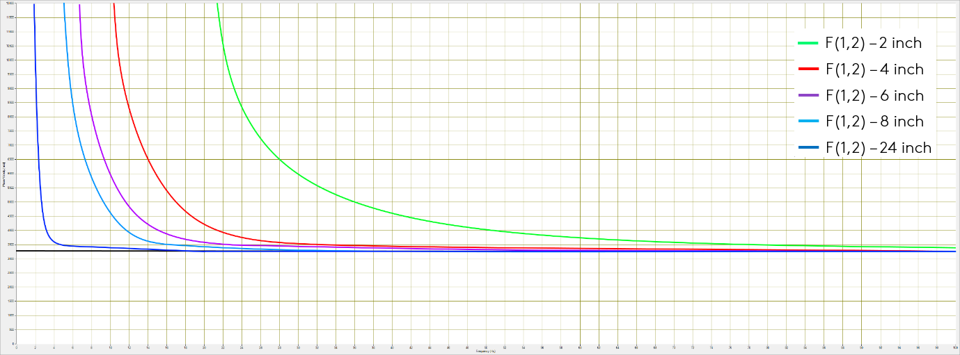 Figure 1: F(1,2) Wave mode at various pipe diameters
The 2in/50mm pipe is the worst-case scenario as many of the lower frequency options (20kHz – 55kHz) are now unavailable. The Wavescan™ software will avoid the collection of these frequencies as a safety net. If we were to choose to collect data within this frequency range, we would experience a reduction in data quality, and potentially some confusing signals, making interpretation more difficult.
Before understanding the effects of dispersion, it is vital to first understand bandwidth.
When selecting a specific frequency for collection, it is essential to understand that the generated pulse contains an envelope of frequencies specific to its bandwidth.
The bandwidth of a frequency is calculated using the following simplified formula: 4f/n, where f = frequency and n = the number of cycles in the pulse. Refer to the following example.
Applying the formula to a 36kHz, ten cycle pulse gives the following:
This bandwidth will be centered on the main lobe, 36kHz +/- 7.2kHz. This ultimately means that the frequency envelope of this pulse will range from 28.8kHz to 43.2kHz, as shown in Figure 2. Figure 2 displays the T(0,1) wave mode and its associated flexural wave mode F(1,2).
It is important to note that the frequency bandwidth of the 36kHz pulse does not affect the T(0,1) wave mode as it is non-dispersive across the entire frequency range. The frequency bandwidth of the pulse will, in this example, affect the F(1,2) wave mode as this wave mode is dispersive within the frequency range stated.
Once the T(0,1) wave mode converts, it produces a dispersive F(1,2) wave mode, as the high frequency components of the pulse travel at approximately 3235m/s and the low frequency components of the pulse travel at around 3195m/s. This will cause the pulse to broaden as it propagates along the pipe.
-at-small-diameters.png)
Figure 2: F(1,2) at small diameters
As Teletest operators, we want to ensure that we obtain the best possible data quality. So, what can we do in the case of inspecting a 2in/50mm pipeline, for example?
We know from the previous information that the flexural mode associated with Torsional testing at this diameter is dispersive; is there anything we can do to minimize these effects?
Yes, there is. If we refer to the bandwidth formula, there is one variable in that formula that we can adjust for a given frequency.
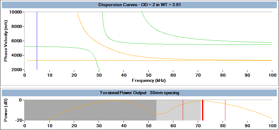
Figure 3: Dispersion and output curves for ten-cycle pulse in 2in/50mm pipe
Figure 3 displays the phase velocity (Vp) dispersion curves and power output curves for a ten-cycle pulse in a 2in/50mm diameter pipe with a 0.15in/3.91mm wall thickness. The shaded (grey) sections on the power output curves show the frequency regions that are undesirable for guided wave tests. The dark grey area indicates frequencies that should not be selected, and the light grey area identifies the frequency range that should be used with caution.
Figure 4 displays the same information as Figure 3; however, the pulse length has been increased to 15 cycles. A definite improvement in the usable frequency range is apparent (note that the light grey shaded area is now below 60kHz in Figure 4, compared to above 70kHz in Figure 3), and the dispersive effects of F(1,2) are also reduced, due to the pulse having a narrower bandwidth.
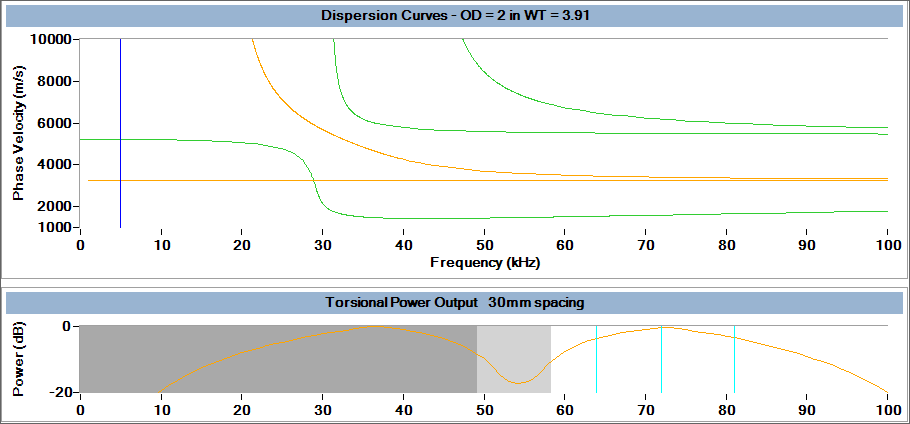
Figure 4: Dispersion and output curves for 15 cycle pulse in 2in/50mm pipe
So, what can we take away from this information? It is clear to see that when testing small diameter pipelines, mainly 2in/50mm, we are likely to see improved data quality with a longer pulse length, as this will reduce bandwidth. The table below gives a summary of the effects of adjusting the pulse length.
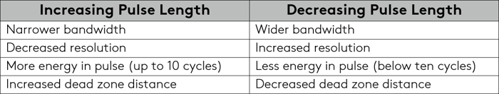
Having a longer pulse length will narrow the bandwidth and therefore reduce the effects of dispersive wave modes; however, that comes at a cost.
A longer pulse also means a decrease in resolution. That’s not an issue in the case of small diameter pipelines as we are testing in a higher frequency range.
Remember a 72kHz fifteen cycle pulse has a better resolution that a 36kHz ten cycles pulse.
When testing small, increase the pulse length.
For more information on the Teletest Focus+™ for your small diameter pipeline inspections, contact our experts today!